Consolidating and Redistributing Excess Capacity in Parcel Locker Networks

Successful out-of-home (OOH) networks require adequate spatial distribution of capacity. Even though this seems trivial, it is not - demand patterns are not static, customer behavior shifts over time, and a network that was well-balanced last year can quietly drift out of shape without a single change made to the network.

When lockers or shops sit close enough together that they're effectively competing for the same customers, keeping all of them running isn't necessarily better than having fewer, better-placed ones. But which ones to remove, and how many, isn't obvious. Remove too aggressively and you lose real coverage, or put surrounding lockers under more pressure than they can handle. Remove too little and you're leaving redundant capacity in place.

‍

Capacity Strain Index

In order to assess whether capacity is sufficient in a given area, several things need tracking at once: each locker or shop's catchment area, its physical capacity, and how long a package typically sits before pickup. None of these are simple on their own. 

Determining demand within a catchment area means accounting for competing lockers nearby. Distance is usually the best predictor of that pull, since the closer a locker sits to a source of demand, the more likely it is to attract it over a competitor. 

Physical capacity isn't a fixed number either. How long packages sit before being collected effectively renders part of that capacity unavailable for the time being, so two lockers with identical shelf space can behave very differently depending on how quickly customers pick up.

Trying to reason about network balance by inspecting each of these separately, location by location, quickly becomes unmanageable - a change in any one factor ripples through several others at once. This is exactly what the Capacity Strain Index (CSI) exists to solve: a single, comparable number per location that collapses catchment overlap, competing demand, physical capacity, and pickup speed together, so that "is this location under strain" becomes a question with one clear answer.

The way we mathematically define CSI is as follows:

For a given locker/shop, Q represents the overall volume of shipments within its catchment area in an observed time period t. It consists of two components: 

• Q _exclusive - shipments exclusive only to the observed locker/shop;
• Q _shared - shipments derived from the portion of the catchment area shared with other lockers/shops within the network.

Q _shared can't simply be split evenly among however many locations compete for it. Splitting shared demand evenly regardless of distance would systematically overstate how much competition a nearby location actually faces, and understate it for the location that's genuinely closer. To account for this, we drew inspiration from the famous Huff model. Each competing location's share of Q _shared is weighted by distance decay: the pull a location exerts on a given area of shared demand falls off the farther away it is. Take a shared area with several competing locations. Each one's share is proportional to some decreasing function of its distance - for example, inverse distance or inverse-squared distance - normalized against the combined pull of every competitor reaching that same area.

t _{dwell average} accounts for how long a parcel typically sits before being picked up. A locker whose parcels are collected quickly can effectively serve more real demand with the same physical capacity than one where parcels linger. Dwell time doesn't change how much capacity exists, but it changes how much of that capacity is genuinely available at any given moment. Capacity itself, in the denominator, is simply how much volume the location can physically hold. 

Together, the formula expresses CSI as demand pressure, adjusted for how quickly that capacity actually turns over, relative to how much capacity is physically available, aligning with Little’s law in queueing theory. A value of 1 represents the point at which demand and effective capacity are perfectly matched. CSI value below 1 indicates overcapacity, while a value above 1 signals undercapacity. One thing to keep in mind is that CSI is asymmetrical - in the overcapacity domain it ranges from 0 to 1 while in the undercapacity range it does not have a right-side limit. 

‍

Finding redundant clusters

Here, we'll demonstrate how CSI can help navigate the process of consolidating capacity by removing redundant lockers and shops in a network.

The general idea behind removing redundant entities is to reduce their number as much as possible while still keeping enough capacity to sufficiently cover demand across the whole affected area. Finding redundancy candidates can be done in several ways.  We used Jaccard similarity, with clustering built on top of it, to identify groups of lockers that make sense to consolidate. The Jaccard similarity index (JSI) is defined as the ratio of the intersection of two sets to their union.

On Mily Tech’s platform, each locker or shop covers a set of hexagons within its catchment area, which makes JSI a natural fit for identifying overlapping capacity. For each pair of locations, JSI is computed, and any pair exceeding a given similarity threshold gets grouped together. In effect, this finds locations that are genuinely competing for the same demand.

The obvious next step looks simple: within each overlapping group, shrink down to just one location and let it absorb everyone else's demand. But this turns out to be the wrong approach. The question "should we consolidate" becomes "consolidate to how many, and does the surviving capacity actually match the new demand?" Sometimes the answer is one location. Sometimes it's two or three. Sometimes it's genuinely best to change nothing at all.

‍

Why removal alone isn't enough

A first intuition might be to shrink a cluster down to however few survivors keep their CSI closest to 1, the ideal value. But clusters rarely exist in isolation. Most have neighboring lockers that share some of the same demand, and any capacity change inside the cluster ripples out to them. Reduce a cluster too aggressively, and its neighbors get overwhelmed by the larger share of shared demand suddenly landing on them. 

This means any capacity reduction inside a cluster requires readjusting capacity in its neighborhood too. That isn't necessarily a bad thing, since it's an opportunity to actively re-tune neighboring lockers to fit the new demand landscape, not just an unwanted side effect to manage. Of course, to make the capacity adjustment realistic, information on whether there is potential for increasing capacity at neighboring locations is required.

Given that, a simple local search aimed at minimizing CSI deviation across both the cluster and its neighborhood turns out to be enough. Usually, undercapacity costs more than overcapacity, therefore the CSI deviation can be penalized differently depending on which side of 1 it falls on. For this experiment, we treat CSI deviation symmetrically regardless of direction. The method checks every possible outcome - from keeping everyone active down to the fewest locations allowed - and measures how well-matched capacity is to demand at each option. Whichever option leaves the network best-balanced is the one chosen.

‍

‍Putting it to the test

We ran this simple heuristic approach on 52 real-life urban area instances. The solution's behavior is tracked against different assumed package dwell times in lockers. To highlight the importance of accounting for capacity adjustment in cluster-neighboring locations, we also introduced a scenario where only the clusters are consolidated, without neighbor awareness.

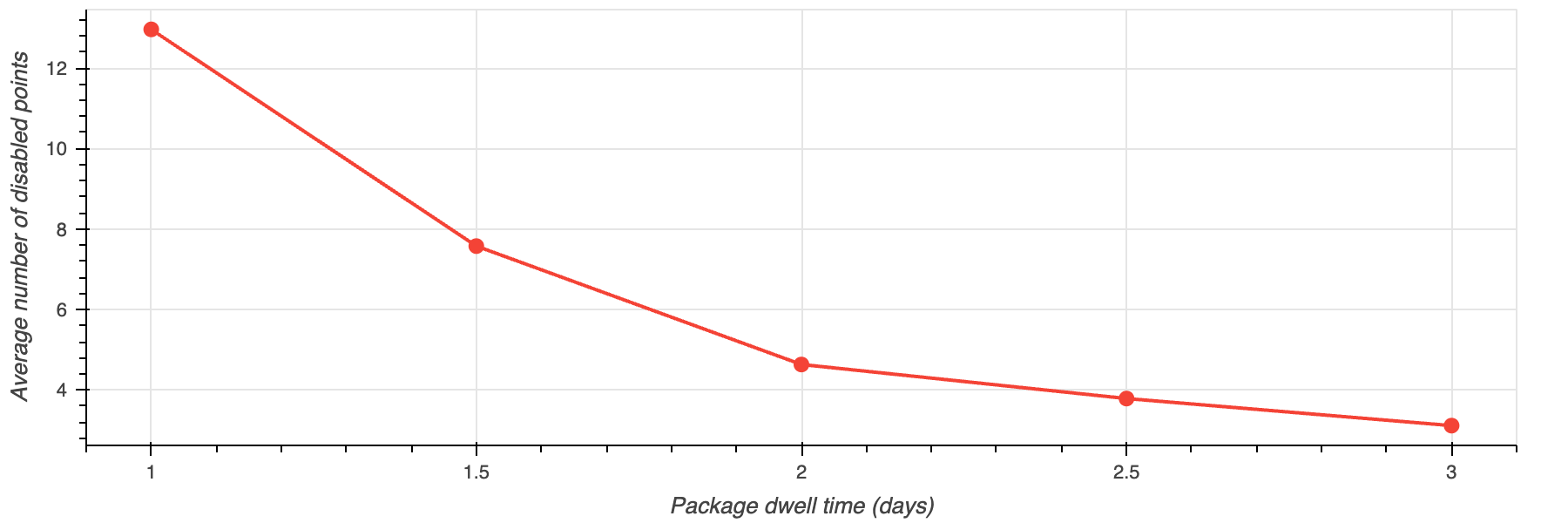
The first sanity checks are shown in the two figures below. The first figure shows the average number of disabled locations per instance relative to the observed dwell time. It's clear that network consolidation has less room to maneuver as average package dwell time rises - yet even so, some locations still get consolidated. This makes sense: the longer the dwell time, the more capacity is actually needed to cover the same amount of demand, which results in fewer locations being disabled.

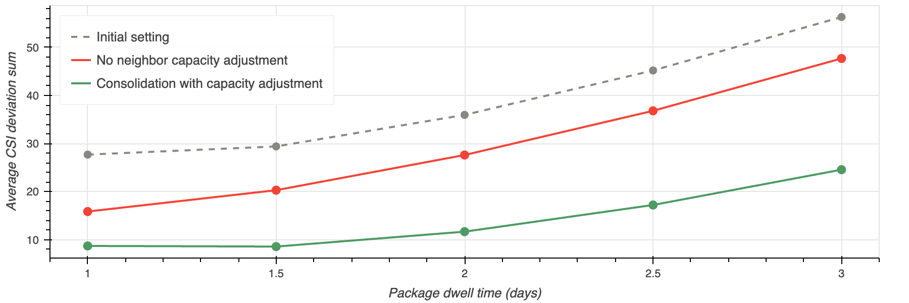
The second figure shows the overall improvement in CSI values across the three scenarios considered - the initial setup, consolidation without neighbor capacity adjustment, and the full heuristic approach that includes it. This is tracked by summarizing each location's individual CSI deviation from 1, the theoretical ideal value. The figure shows that while raw consolidation alone does improve CSI, the full effect is only achieved when consolidation is accompanied by capacity readjustment.

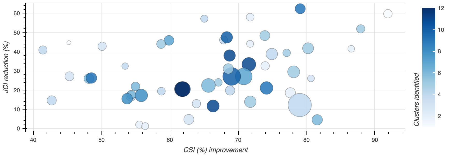
Of course, we won't let CSI alone make the case that the solution has genuinely improved. The figure below shows that, across all instances, consolidation reduced the average Jaccard similarity - meaning locations end up more evenly spread out in space. The Jaccard similarity is a cheap geometric proxy for the demand overlap that cannibalization measures directly, so removing overlapping locations naturally reduced cannibalization as well. The largest CSI improvements are achieved in instances with the highest cannibalization rate - that is, the greatest overlap between locations' catchment areas. Interestingly, the amount of CSI/JCI improvement is not correlated with the number of identified clusters. This means that the potential for improvement lies in the number of tightly packed locations, rather than in the number of groups.

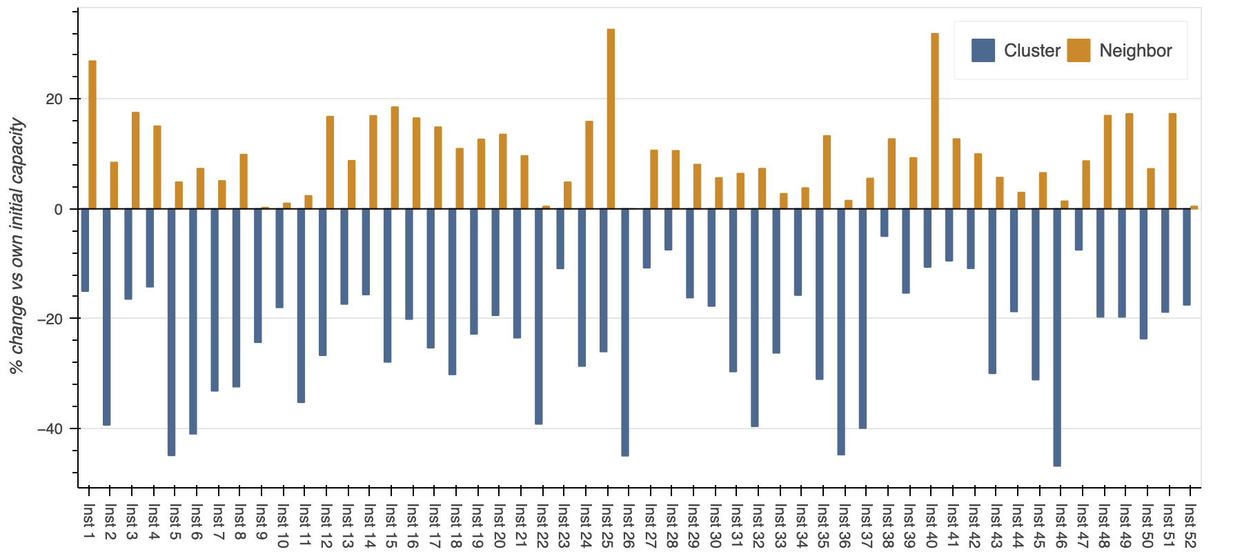
The general redistribution of capacity shows the overall overcapacitation of the initial network setup - more capacity is removed from clusters than is added to neighboring locations. This shows the heuristic resolves two issues at once: it redistributes capacity where needed, and it removes unnecessary capacity from the network altogether.

‍

The takeaway 

What this experiment ultimately shows is that CSI turns a genuinely tedious, multi-factor decision into a single value a simple heuristic can use as guidance. Its usefulness is demonstrated on the problem of consolidating redundant capacity in OOH networks.

Regarding the capacity consolidation itself - identifying and removing redundant locations is the obvious half of the problem, but getting the surrounding network to actually fit to the new demand landscape is the half that matters. This is backed up by the results showing that only after neighbor capacity readjustment the full effect of removing redundant capacity is achieved.

‍This is part of ongoing research at Mily Tech into network optimization. If you're interested in solving similar problems like this one, reach out at research@milytech.com. We'd love to collaborate.